Independent samples t test: choosing, interpreting and reporting Welch
Interpret a two-group Welch t test, mean differences, confidence intervals and effect size using a complete study with traceable data and outputs.
First decide whether the observations are independent
An independent samples t test addresses a difference between two population means using observations from separate groups. Two columns do not necessarily mean two independent samples. Before-and-after measurements on the same people form pairs; their dependence must be retained in the analysis. The official R t-test documentation distinguishes paired and unpaired analyses.
The advanced research example compares work engagement between employees in hybrid and onsite arrangements. Each employee contributes one record. There was no random assignment, so a group difference is an observed association rather than evidence that changing work arrangement causes a change in engagement. The test-selection guide puts this decision in the wider study design.
Understand which t test was reported
Welch's test estimates variability separately for the two groups rather than assuming equal population variances. Its degrees of freedom can be fractional; that value is not the number of participants. NIST gives the two-sample formulas, including the Welch–Satterthwaite approximation. The pooled-variance version uses a different standard error and degrees of freedom.
In this example, the reported H3 analysis uses Welch's test with a two-sided alternative. Do not switch to a one-sided test after looking at the observed direction, or copy a pooled-test row while calling it Welch. Investigate the data structure, unusual observations and distribution; a normality-test p value alone does not establish independence or justify deleting records.
Worked comparison: engagement by work arrangement
The following summaries were recalculated from the published prepared data. Engagement is the mean of five items scored from 1 to 5, with no missing values in this example.
גללו לצדדים לצפייה בכל העמודות ↔Scroll sideways to view all columns ↔
| Group | n | Mean | SD |
|---|---|---|---|
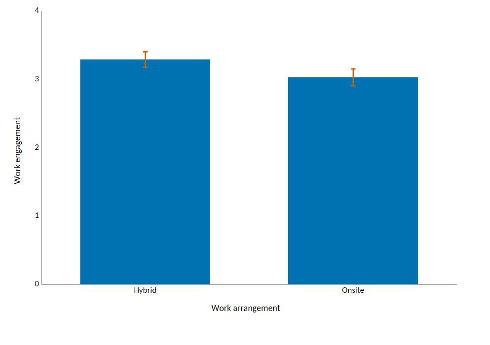
| Hybrid | 185 | 3.29 | 0.78 |
| Onsite | 175 | 3.03 | 0.83 |
Define the difference explicitly as hybrid minus onsite. It is 0.260 score points, with a 95% confidence interval of approximately [0.092, 0.428] points. The Welch statistic is t(353.17) = 3.05, with an unadjusted two-sided p value of approximately .00250, reported as .003 when rounded to three decimals. Using rounded group means to recompute the test can produce slightly different results; calculations use the unrounded values.
This interval concerns the mean difference under the analysis assumptions, not the range containing 95% of employees' individual scores. Reversing the group order reverses the sign of the difference and t statistic, and changes the interval's orientation. It does not change the two-sided p value.
Keep score points, effect size and adjusted p values separate
The existing output also reports Hedges' g = 0.32, with a 95% interval of approximately [0.11, 0.53]. This is a standardized mean difference, not 0.32 engagement-score points or a percentage. The effectsize documentation explains standardized differences and alternative standardization choices. Identify the reported measure rather than treating every effect-size column as interchangeable.
The interval for g and the interval for the mean difference use different scales. Label them separately. The example's analysis plan groups H1–H3 into a confirmatory family with Holm adjustment; the complete findings chapter reports the adjusted p value alongside the raw p value. Both round to .003 for H3. An unadjusted interval for one contrast is not automatically a simultaneous interval for all hypotheses in the family.
A clear reporting paragraph
“Mean engagement was 3.29 (SD = 0.78) in the hybrid group (n = 185) and 3.03 (SD = 0.83) in the onsite group (n = 175). Welch's two-sided t test gave t(353.17) = 3.05, p = .003. The hybrid-minus-onsite mean difference was 0.260 points, 95% CI [0.092, 0.428]. Hedges' g was 0.32, 95% CI [0.11, 0.53]. The Holm-adjusted p value was also .003 when rounded. Work arrangement was not randomly assigned, so no causal effect is inferred.”
Adapt the wording to the actual question, scoring and analysis plan. A non-significant difference would not, by itself, establish equivalence. Statistical significance also does not tell you whether a difference matters in the study's context.
Follow the decision back to the files
Inspect the study description, variable dictionary, precise results and decision record. H3 compares the groups without covariate adjustment. The additional A1 regression asks a conditional question with other predictors; its coefficient is not the same estimand as this raw group contrast. The regression guide explains that distinction.
See the statistical analysis service for possible deliverables within an agreed scope. Consultation and ordering remain closed; service availability shows the current status.
See the complete research examples
Follow the research questions through the input files, analysis plan and outputs. Each example includes the consultation report, itemized illustrative price and generated files.
Basic example · undergraduate level
Academic self efficacy and learning persistence
A questionnaire study with two scales and one association hypothesis: reliability, descriptive statistics and a Pearson correlation.
Advanced example
Job autonomy, supervisor support and work engagement
A three-scale study with factor analysis, reliability, three hypotheses including regression, and an additional background-adjusted model.